- Introduction
- How to analyse an algorithm?
- Asymptotic Analysis
- Asymptotic Notations
- Rate of Growth
- Amortized Analysis
- Iterative Algorithm Analysis
- Recursive Algorithm Analysis
Introduction
Algorithm vs Programs
- Algorithm - Design, requires Domain Knowledge, Any Language, Hardware and Software independent, Analyze phase.
- Programs - Implementation, Programmer, Programming Language, Hardware and Software Dependent, Testing phase.
Priori Analysis vs Posteriori Testing
- Priori Analysis - for Algorithm, Language independent, Hardware independent, in terms of Time and Space Function
- Posteriori Testing - for Programs, Language dependent, Hardware dependent, Watch time and bytes
How to analyse an algorithm?
- Time
- Space
- Network consumption
- Power
- CPU Registers consumed (driver development)
Why? - All things (user friendliness, modularity, security, maintainability, etc) depends on performance.
Given two algorithms for a task, how do we find out which one is better?
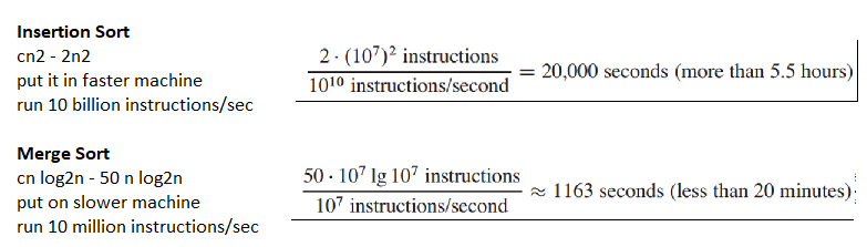
- Naive way – implement both and run them for different inputs and see which one takes less time.
- Asymptotic Analysis There are many problems with this approach for analysis of algorithms:
- There can be many sets of input
- For some inputs, 1st algorithm performs better than the second and vice-versa – (binary vs linear search)
- For some inputs, 1st algorithm performs better on one machine and vice-versa.
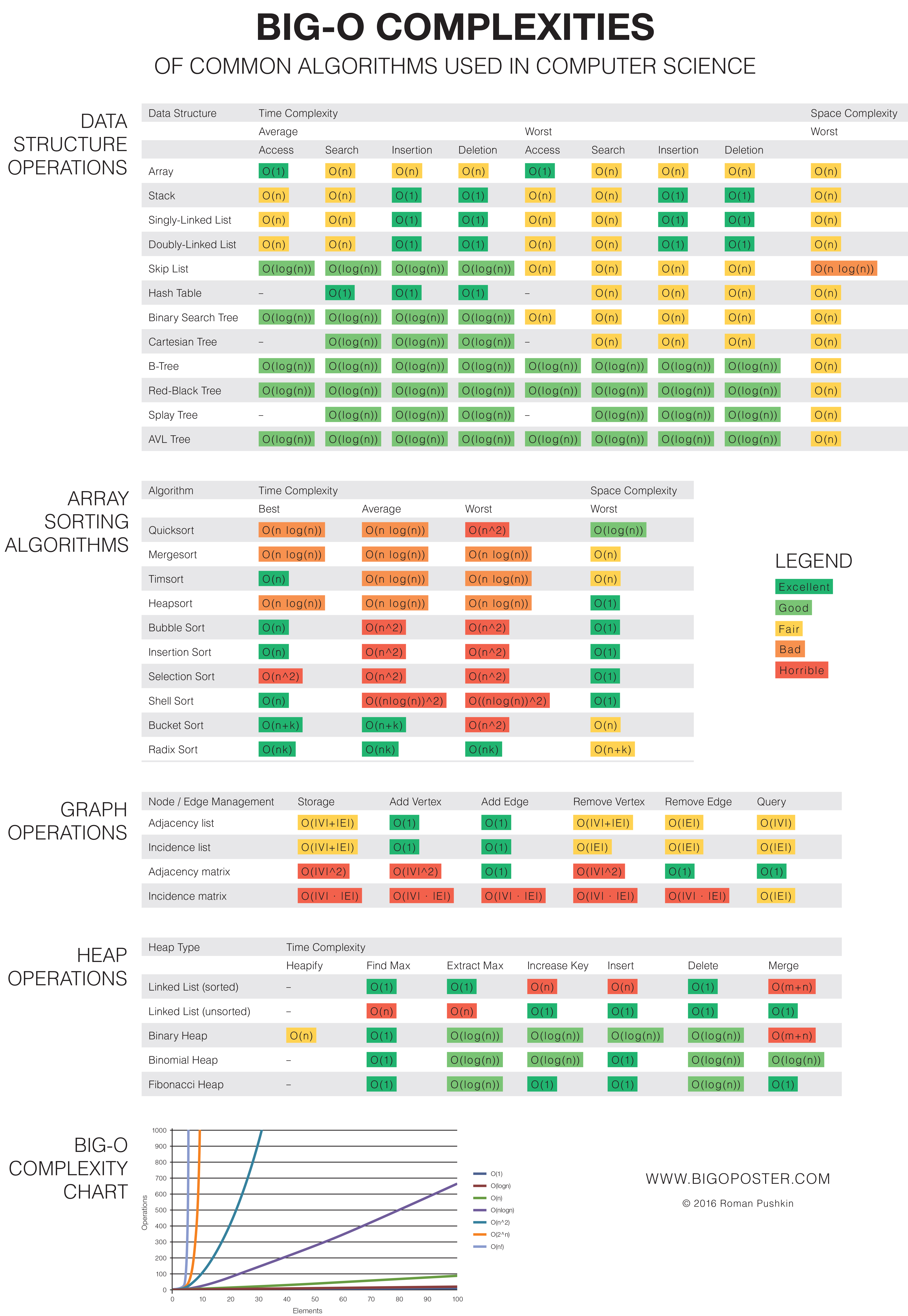
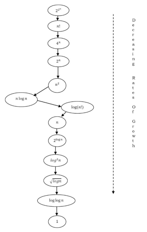
lg n < n^0.5 < n < n lg n < n^2 < n^3 <2^n < n!
Asymptotic Analysis
Asymptotic Analysis
- Evaluate performance of an algorithm in terms of input size (not actual running time).
- Calculate how does the time (or space) taken by an algorithm increases with the input size.
Does Asymptotic Analysis always work?
- we always talk about input sizes larger than a constant value.
- If such large input never given, we may end up choosing an algorithm that is Asymptotically faster but slower for our specific requirement.
- Algorithms 1000nLogn, 2nLogn asymptotically same (order of growth is nLogn). can’t judge as we ignore constants.
Space Complexity
- Auxiliary Space, extra space or temporary space used by an algorithm.
- Space Complexity, (Auxiliary space + space used by input) = (total space taken with respect to input size)
- Example, compare standard sort algorithms based of space, Auxiliary Space is better criterion than Space Complexity.
- Merge Sort - O(n) auxiliary space
- Insertion sort - O(1) auxiliary space
- Heap Sort use - O(1) auxiliary space
- but all have Space complexity O(n).
Worst Case Analysis (Usually Done)
- Calculate upper bound, case that causes maximum number of operations to be executed.
- Linear Search, when the element to be searched is not present in the array. O(n).
Average Case Analysis (Sometimes done)
- All possible inputs and calculate computing time for all of the inputs.
- Sum all calculated values and divide by total number of inputs. We must know (or predict) distribution of cases.
- Linear Search, assume all cases are uniformly distributed (also x not present).
Best Case Analysis (Bogus)
- Calculate lower bound, case that causes minimum number of operations to be executed.
- Linear Search, when x is present at the first location. Θ(1).
| Merge Sort | Cases | all the cases are asymptotically same, i.e., there are no worst and best cases. Merge Sort does Θ(n logn) operations in all cases. |
| Insertion sort | Worst | when the array is reverse sorted |
| Best | when the array is sorted in the same order as output. | |
| Quick Sort | Worst | when the input array is already sorted. (where pivot is chosen as a corner element) |
| Best | when the pivot elements always divide array in two halves. |
Asymptotic Notations
- Asymptotic Analysis - To have a measure of efficiency of algorithms indepent of machine-specific constants without implementing the algorithm.
- Asymptotic Notations - Mathematical tools to represent time complexity of algorithms for asymptotic analysis.
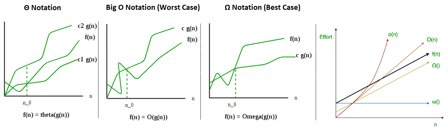
Θ Notation:
- Bounds a function from above and below, so it defines exact asymptotic behavior.
- 3n^3 + 6n^2 + 6000 = Θ(n^3), there will always be a number n0 after which Θ(n^3) has higher values than Θn^2) irrespective of the constants involved.
Θ(g(n)) = { f(n): there exist positive constants c1, c2 and n0
such that 0 <= c1*g(n) <= f(n) <= c2*g(n) for all n >= n0 }
The above definition means,
- if f(n) is Θ(g(n)), then the value f(n) is always between c1g(n) and c2g(n) for large values of n (n >= n0).
- f(n) must be non-negative for values of n greater than n0.
Big O Notation (Worst Case)
- Defines an upper bound of an algorithm, it bounds a function only from above.
- If we use Θ notation to represent time complexity of Insertion sort, we have to use two statements for best and worst cases:
- The best-case time complexity of Insertion Sort is Θ(n).
- The worst-case time complexity of Insertion Sort is Θ(n2), also covers linear time.
Useful when we only have upper bound on time complexity of an algorithm.
O(g(n)) = {f(n): there exist positive constants c and n0
such that 0 <= f(n) <= cg(n) for all n >= n0}
Ω Notation (Best Case)
Ω notation provides an asymptotic lower bound, best-case performance and least used notation.
For a given function g(n), we denote by Ω(g(n)) the set of functions.
Ω (g(n)) = {f(n): there exist positive constants c and n0
such that 0 <= cg(n) <= f(n) for all n >= n0}.
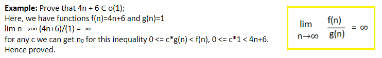
Little ο asymptotic notation
- Little o provides strict upper bound (equality condition is removed from Big O)
- Big-Ο (O(n)) is used as a tight upper-bound.
- Little-ο (ο(n)) notation is used for loose upper-bound.
Let f(n) and g(n) be functions that map positive integers to positive real numbers.
f(n) = ο(g(n)) OR ο(g(n)) = { f(n): there exist positive constants c > 0, n0 > 1
such that 0 <= f(n) < c.g(n)  for all n > n0 }

Little ω asymptotic notation
- Little omega provides strict lower bound (equality condition removed from big omega)
Let f(n) and g(n) be functions that map positive integers to positive real numbers.
f(n) = ω(g(n)) OR ω(g(n)) = { f(n): there exist positive constants c > 0, n0 ≥ 1
such that f(n) > c.g(n) ≥ 0  for all n > n0 }
- Symbolises Loose lower bound.
- f(n) has a higher growth rate than g(n).
For Big Omega f(n)=Ω(g(n)), bound is 0<=c*g(n0), For little omega, it is true for all constant c>0.
f(n) = ω(g(n)) if and only if g(n) = ο((f(n)).
Rate of Growth
Acceptable
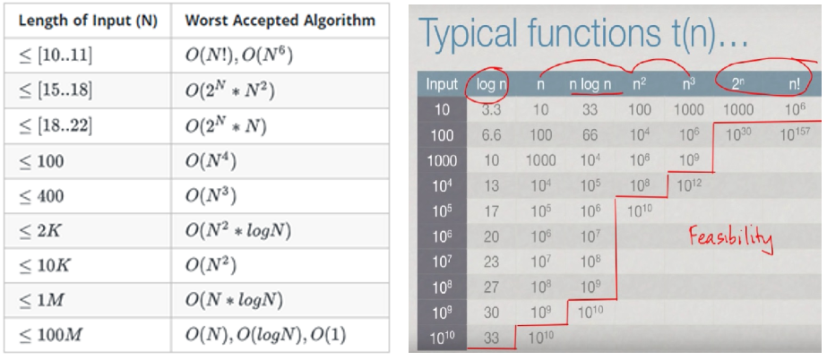
Order Rate of Growth
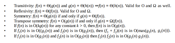
Asymptotic Notations Properties
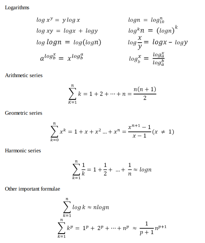
Common Summation and Series
Amortized Analysis
- Used for algorithms where an occasional operation is very slow, but most of the other operations are faster.
- In Amortized Analysis, we analyze a sequence of operations and guarantee a worst-case average time which is lower than the worst-case time of a particular expensive operation.
- The example data structures whose operations are analyzed using Amortized Analysis are Hash Tables, Disjoint Sets and Splay Trees.
Let us consider an example of a simple hash table insertions. How do we decide table size?
- There is a trade-off between space and time, if we make hash-table size big, search time becomes fast, but space required becomes high.
- The solution to this trade-off problem is to use Dynamic Table (or Arrays). The idea is to increase size of table whenever it becomes full. Following are the steps to follow when table becomes full.
- Allocate memory for a larger table of size, typically twice the old table.
- Copy the contents of old table to new table.
- Free the old table. If the table has space available, we simply insert new item in available space.
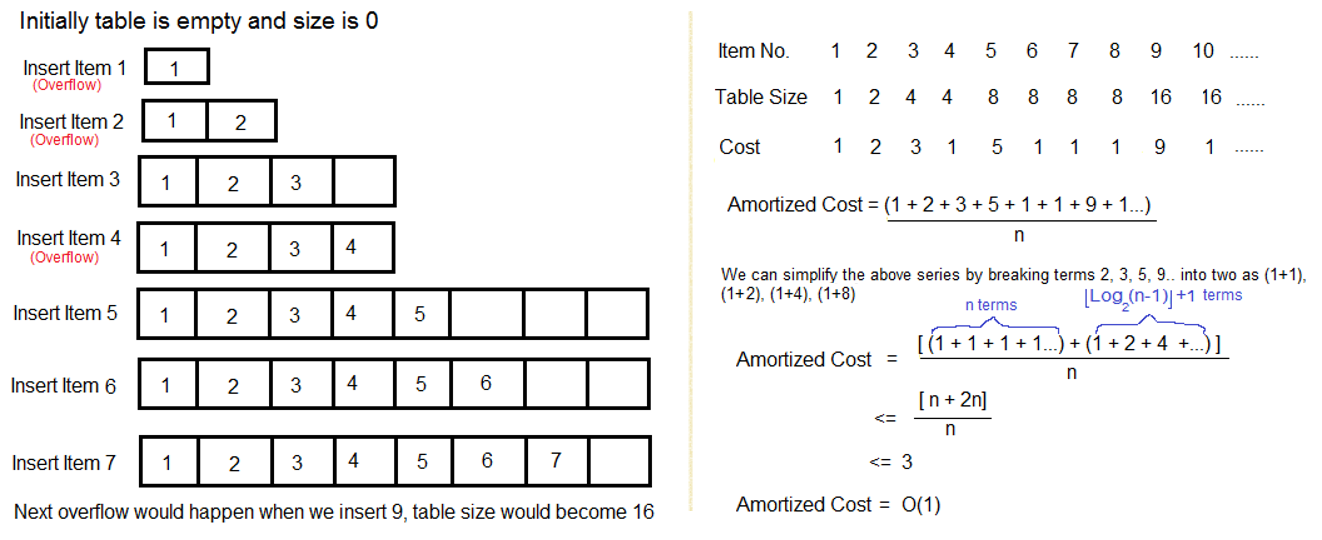
What is the time complexity of n insertions using the above scheme? If we use simple analysis, the worst-case cost of an insertion is O(n). Therefore, worst case cost of n inserts is n * O(n) which is O(n2). This analysis gives an upper bound, but not a tight upper bound for n insertions as all insertions don’t take Θ(n) time.
So using Amortized Analysis, we could prove that the Dynamic Table scheme has O(1) insertion time which is a great result used in hashing. Also, the concept of dynamic table is used in vectors in C++, ArrayList in Java.
Following are few important notes.
- Amortized cost of a sequence of operations can be seen as expenses of a salaried person. The average monthly expense of the person is less than or equal to the salary, but the person can spend more money in a particular month by buying a car or something. In other months, he or she saves money for the expensive month.
- The above Amortized Analysis done for Dynamic Array example is called Aggregate Method. There are two more powerful ways to do Amortized analysis called Accounting Method and Potential Method. We will be discussing the other two methods in separate posts.
- The amortized analysis doesn’t involve probability. There is also another different notion of average case running time where algorithms use randomization to make them faster and expected running time is faster than the worst-case running time. These algorithms are analyzed using Randomized Analysis. Examples of these algorithms are Randomized Quick Sort, Quick Select and Hashing. We will soon be covering Randomized analysis in a different post.
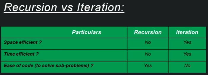
Iterative Algorithm Analysis
- Algorithms can be Iterative or recursive.
- Here performance (running time) depends on the input-size.
- If neither iterative nor recursive then its O(1), constant time.
- Hence no dependency on input-size.
- Program written using iteration can also be written in recursive and vice-versa.
O(1)
- Time complexity of a function (or set of statements) is considered as O(1) if it doesn’t contain loop, recursion and call to any other non-constant time function.
- For example swap() function has O(1) time complexity.
- A loop or recursion that runs a constant number of times is also considered as O(1).
for (int i = 1; i <= c; i++) { // Here c is a constant
// some O(1) expressions
}
O(n):
- Time Complexity of a loop is considered as O(n) if the loop variables are incremented / decremented by a constant amount.
for (int i = 1; i <= n; i += c) { // Here c is a positive integer constant
	// some O(1) expressions
}
O(n^c)
- Time complexity of nested loops is equal to the number of times the innermost statement is executed.
- For example, Selection sort and Insertion Sort have O(n^2) time complexity.
- For example, the following sample loops have O(n^2) time complexity.
for (int i = 1; i <=n; i += c) {
    for (int j = 1; j <=n; j += c) { // some O(1) expressions }
}
O(Logn)
Time Complexity of a loop is considered as O(Logn) if the loop variables is divided / multiplied by a constant amount.
for (int i = 1; i <=n; i *= c) {
    // some O(1) expressions
}
- For example Binary Search(refer iterative implementation) has O(Logn) time complexity.
- Let us see mathematically how it is O(Log n). The series that we get in first loop is 1, c, c2, c3, … ck. If we put k equals to Logcn, we get c^(Logcn) which is n.
O(LogLogn)
Time Complexity of a loop is considered as O(LogLogn) if the loop variables is reduced / increased exponentially by a constant amount.
for (int i = 2; i <=n; i = pow(i, c)) {  // Here c is a constant greater than 1
    // some O(1) expressions
}
for (int i = n; i > 0; i = fun(i)) {/* some O(1) expressions */}
//Here fun is sqrt or cuberoot or any other constant root
How to combine time complexities of consecutive loops?
- When there are consecutive loops, we calculate time complexity as sum of time complexities of individual loops.
for (int i = 1; i <=m; i += c) { /* some O(1) expressions */ }
for (int i = 1; i <=n; i += c) { /* some O(1) expressions */ }
- Time complexity of above code is O(m) + O(n) which is O(m+n)
- If m == n, the time complexity becomes O(2n) which is O(n).
How to calculate time complexity when there are many if, else statements inside loops?
- Mostly Worst case time complexity is useful, We evaluate the situation when values in if-else conditions cause maximum number of statements to be executed.
- For example consider the linear search function where we consider the case when element is present at the end or not present at all. When the code is too complex to consider all if-else cases, we can get an upper bound by ignoring if else and other complex control statements.
i=1; s=1
While(s<=n){
    i++;    // I -> 1 2 3 4  5  6
    s=s+i;  // s -> 1 3 6 10 15 21
}

This is sum of natural numbers series. (k(k+1)/2) > n
k = O{sqrt(n)}
Recursive Algorithm Analysis
- Recursive algorithms are have a recurrence relation for time complexity.
- We get running time on an input of size n as a function of n and the running time on inputs of smaller sizes.
- For example in Merge Sort, to sort a given array, we divide it in two halves and recursively repeat the process for the two halves. Finally we merge the results.
- Time complexity of Merge Sort can be written as
T(n) = 2T(n/2) + cn.
- Time complexity of Merge Sort can be written as
- There are many other algorithms like Binary Search, Tower of Hanoi, etc.
There are mainly three ways for solving recurrences:
- Substitution Method
- Recurrence Tree Method
- Master Method
Substitution Method
- We make a guess for the solution and then we use mathematical induction to prove the guess is correct or incorrect.
- For example consider the recurrence T(n) = 2T(n/2) + n
- We guess the solution as T(n) = O(nLogn). Now we use induction to prove our guess.
- We need to prove that T(n) <= cnLogn. We can assume that it is true for values smaller than n.
T(n) = 2T(n/2) + n <= cn/2Log(n/2) + n
    =  cnLogn - cnLog2 + n
    =  cnLogn - cn + n
    <= cnLogn
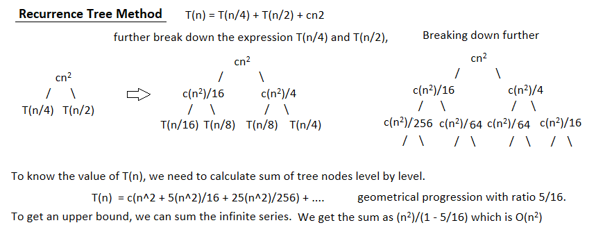
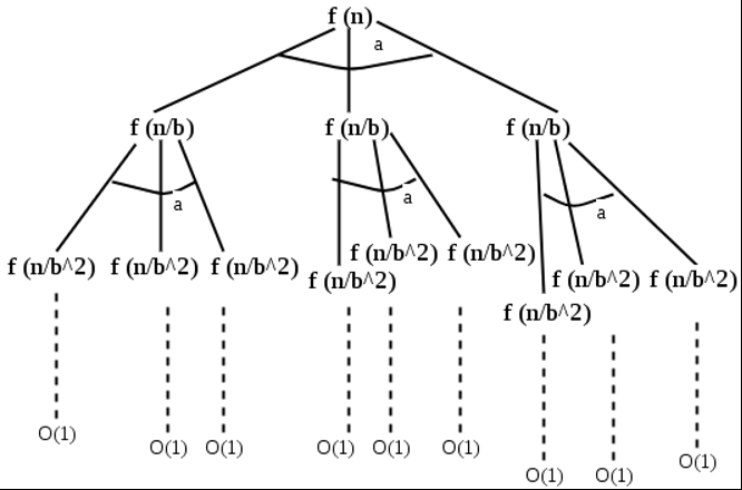
Recurrence Tree Method:
- In this method, we draw a recurrence tree and calculate the time taken by every level of tree.
- Finally, we sum the work done at all levels.
- To draw the recurrence tree, we start from the given recurrence and keep drawing till we find a pattern among levels.
- The pattern is typically a arithmetic or geometric series.
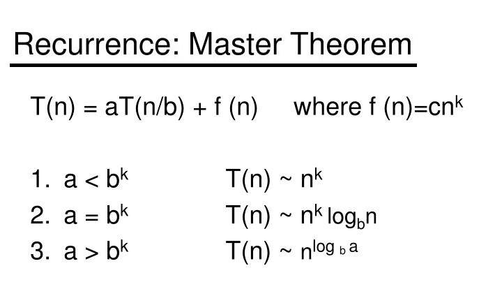
Master Method:
- Master Method is a direct way to get the solution.
- The master method works only for following type of recurrences or for recurrences that can be transformed to following type.
How does this work?
- Master method is mainly derived from recurrence tree method.
- If we draw recurrence tree of
T(n) = aT(n/b) + f(n), we can see that the work done at root is f(n) and work done at all leaves is Θ(nc) where c is Logba. And the height of recurrence tree is Logbn.
In recurrence tree method, we calculate total work done.
- If the work done at leaves is polynomially more, then leaves are the dominant part, and our result becomes the work done at leaves (Case 1).
- If work done at leaves and root is asymptotically same, then our result becomes height multiplied by work done at any level (Case 2).
- If work done at root is asymptotically more, then our result becomes work done at root (Case 3).
Examples of some standard algorithms whose time complexity can be evaluated using Master Method
- Merge Sort: T(n) = 2T(n/2) + Θ(n). It falls in case 2 as c is 1 and Logba] is also 1. So, the solution is Θ(n Logn)
- Binary Search: T(n) = T(n/2) + Θ(1). It also falls in case 2 as c is 0 and Logba is also 0. So, the solution is Θ(Logn).
Notes:
- It is not necessary that a recurrence of the form T(n) = aT(n/b) + f(n) can be solved using Master Theorem. The given three cases have some gaps between them.
- For example, the recurrence T(n) = 2T(n/2) + n/Logn cannot be solved using master method.
- Case 2 can be extended for f(n) = Θ(n^c (Log n)^k)
- If f(n) = Θ(n^c (Log n)^k) for some constant k >= 0 and c = (Log a/Log b), then T(n) = Θ(n^c (Log n)^(k+1))
Recurrence Relations
Type 1: Divide and conquer recurrence relations
Following are some of the examples of recurrence relations based on divide and conquer.
T(n) = 2T(n/2) + cn
- These types of recurrence relations can be easily solved using master method (Put link to master method).
- For recurrence relation T(n) = 2T(n/2) + cn, the values of a = 2, b = 2 and k =1. Here logb(a) = log2(2) = 1 = k. Therefore, the complexity will be Θ(nlog2(n)).
T(n) = 2T(n/2) + √n
Similarly, for recurrence relation T(n) = 2T(n/2) + √n, the values of a = 2, b = 2 and k =1/2. Here logb(a) = log2(2) = 1 > k. Therefore, the complexity will be Θ(n).
Type 2: Linear recurrence relations
T(n) = T(n-1) + n for n>0 and T(0) = 1
These types of recurrence relations can be easily solved using substitution method (Put link to substitution method). For example,
- T(n) = T(n-1) + n = T(n-2) + (n-1) + n = T(n-k) + (n-(k-1))….. (n-1) + n Substituting k = n, we get
- T(n) = T(0) + 1 + 2+….. +n = n(n+1)/2 = O(n^2)
Type 3: Value substitution before solving
Sometimes, recurrence relations can’t be directly solved using techniques like substitution, recurrence tree or master method. Therefore, we need to convert the recurrence relation into appropriate form before solving. For example,
T(n) = T(√n) + 1
To solve this type of recurrence, substitute n = 2^m as:
T(2^m) = T(2^m /2) + 1
Let T(2^m) = S(m), S(m) = S(m/2) + 1
Solving by master method, we get
S(m) = Θ(logm)
As n = 2^m or m = log2(n),
T(n) = T(2^m) = S(m) = Θ(logm) = Θ(loglogn)
What is the time complexity of Tower of Hanoi problem?
- T(n) = O(sqrt(n))
- T(n) = O(n^2)
- T(n) = O(2^n)
- None
Solution: For Tower of Hanoi,
T(n) = 2T(n-1) + c for n>1 and T(1) = 1.
// Solving this,
T(n) = 2T(n-1) + c
     = 2(2T(n-2)+ c) + c  = 2^2*T(n-2) + (c + 2c)
     = 2^k*T(n-k) + (c + 2c + .. kc)
Substituting k = (n-1), we get
T(n) = 2^(n-1)*T(1) + (c + 2c + (n-1)c) = O(2^n)
Consider the following recurrence: T(n) = 2 * T(ceil (sqrt(n) ) ) + 1, T(1) = 1, Which one of the following is true?
- T(n) = (loglogn)
- T(n) = (logn)
- T(n) = (sqrt(n))
- T(n) = (n)
Solution: To solve this type of recurrence, substitute n = 2^m as:
T(2^m) = 2T(2^m /2) + 1
Let T(2^m) = S(m), S(m) = 2S(m/2) + 1
// Solving by master method, we get
S(m) = Θ(m)
As n = 2m or m = log2n,
T(n) = T(2^m) = S(m) = Θ(m) = Θ(logn)